Assignment: Stochastic Simulation

Problem 1:  The Schlogl Model

This model is famous for its bi-stable steady-state distribution. The reactions are

where B₁ and B₂ denote buffered species whose respective molecular populations N₁ and N₂ are assumed to remain essentially constant over the time interval of interest. There is only one time-varying species, X; the state change vectors are ?₁ = ?₃ = 1, ?₂ = ?₄ = -1; and the propensity functions   are

a₁(x) = (c₁/2) N₁x(x – 1),

a₂(x) = (c₂/6) x(x – 1)(x – 2),                        (2)

a₃(x) = c₃N₂,

a₄(x) = c₄x.

For some values of the parameters this model has two stable states, and that is the case for the parameter values we have chosen here:

c₁ = 3 × 10-7, c₂ = 10^-4, c₃ = 10^-3, c₄ = 3.5, N₁ = 1 × 10⁵, N₂ = 2 × 10⁵.              (3)

Please write a matlab code and run it on octave online. Please plot the trajectories of x when you start from x = 100, 250 and 500 respectively. Then please modify my SSA code to simulate this system with initial value x = 250, plot four trajectories from your simulation to demonstrate that in the stochastic simulation, the system will get quite different results because of randomness. In  your  simulation,  always  use  the  final  simulation  time T  = 6.

Problem 2: Oscillating Gene Expression Model

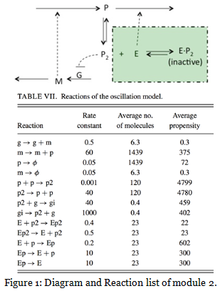
Use your ODE and SSA codes to generate and plot a trajectory for the following oscillating system shown in Figure 1 with the initial conditions: g (gene) = 1; m (mRNA) = 10; p (protein) = 1000; p2 (protein dimer) = 100;    gi (inhibited gene) = 0; E (enzyme) = 100; Ep (enzyme protein complex) =    0; Ep2 (enzyme protein dimer complex)= 0. and final time T = 500.

Attachment:- Biology Assignment.zip